Excel Match Function

Excel Match Function

The Excel MATCH function used to Compare Two Columns of Data

The Excel match function returns the position of a specified value within a column of data.
Its syntax is:
=MATCH(lookup_value,lookup_array,[match_type])

The lookup_array is a column of data values which may or may not be sorted in alphanumeric order. The lookup_value may be either text or numeric.

The optional match_type argument is either 1, 0 or -1 with a default value of 1. If equal to 1, then the column must be sorted in ascending order. In the example below, the formula in D2 reads =MATCH(D1,A1:A8). It correctly returns 6 as the position of the specified value, “Lucy”.

If a non-existent value is used as the lookup, then Excel does an approximate match, returning the position of the previous entry, in alphabetical order. If lookup_value is changed to “Lucia” then 5 is returned, as “Lucy” is later than this value when in alphabetical order; hence Excel returns the position of the previous entry, “Laura”.

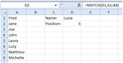
A similar approach is taken if match_type equals -1, except that here the column should be sorted in descending order:

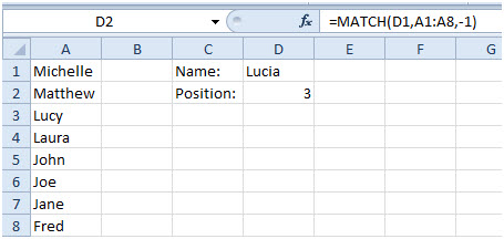
Here “Laura” is earlier than “Lucia”, so Excel returns the position of the entry immediately prior to “Laura”, notably 3.

This “approximate” range lookup can be switched off by setting match_type to zero. If this is the case, then the data may be in any order and #N/A is returned if no match is found:

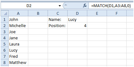
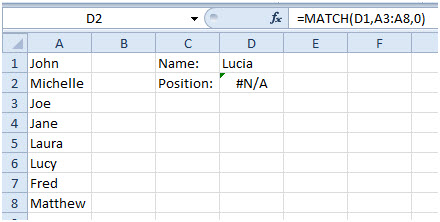
This can be useful in checking whether or not a specified value is located anywhere in a particular data column. It can be combined with the ISNA function.

ISNA takes a formula (or a cell containing a formula) as its sole argument and returns True or False, dependent on whether the #N/A error is returned by the formula or not. Hence it may be used as the logical test in an IF statement:

This can be taken a step further still to compare two columns and, for one column, return YES/NO as to whether there is a match in another column. The two columns do not have to be in the same worksheet. It is also useful to use a range name for the column where the looking up is being done (A1:A8 in this case) as, when copied, the range name will act like absolute cell addresses and will not change.

In the example below, the lookup range has been named using its column heading. To do this, select the range A1:A9 and choose Formulas>Defined Names>Create from selection:

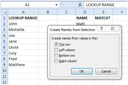
This will name A2:A9 “LOOKUP_RANGE”. To check this, click the drop-down arrow by the name box, and choose “LOOKUP_RANGE”. A2:A9 should be selected:

The column of entries for checking is set up:

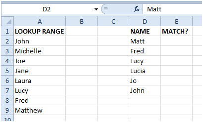
The following formula is entered into E2
=IF(ISNA(MATCH(D2,LOOKUP_RANGE,0)),”NO”,”YES”)

You will find that, when writing a formula, if you select a range that has been named, then Excel will insert the range name, in this case “LOOKUP_RANGE” into the formula. Alternatively the range name can be entered by selecting Formulas>Defined Names>Use in formula: and choosing from the drop-down list of range names in the workbook.

The formula should then be copied down the column. The range name will not change in the copied formula.

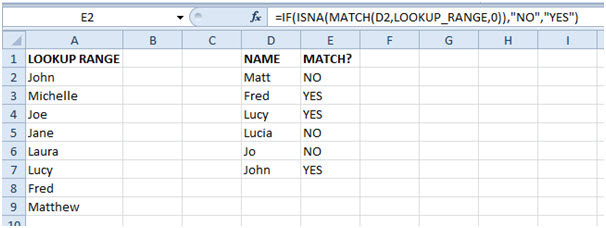
If extra names are added to the Lookup Range column, then the area referenced by the LOOKUP_RANGE can be redefined. If such names are added within the boundaries of the range, i.e. within A2:A9, then Excel will do this automatically. If they are tagged on at the end, then you will need to use the Name Manager to redefine the range’s area:

Select Formulas>Defined Names>Name Manager:

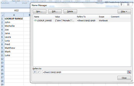
Enter the new range address (in this case just change “A9” to “A11”), click the tick button and close the dialogue box.